Everybody wants to love Reinforcement Learning (RL)! It was the 3rd most popular topic at NeurIPS 2024, just after CV and NLP 🤯! RL has this elegant mathematical framework that mirrors how we humans learn through trial and error. I even identify as an RL person! But in the realm of robotics, RL often feels like trying to fit a square peg in a round hole.

Lately, a new contender—Behavior Cloning (BC)—has swooped in and casually solved tasks that have stumped RL for decades. I recently dipped my toes into BC and want to share why I think it succeeds in tasks where RL fails.

Table of contents

• What can RL do?
• What can RL not do?
• The beautiful simplicity of BC
• Out of distribution
• Conclusion
• References

What can RL do?

Everybody wants to love RL! It is mathematically elegant and follows our real-world intuition. It mimics how we humans learn by trial and error and follows concepts from psychology about reward and punishment. At its core, an RL problem is often formulated as some flavor of Markov Decision Process (MDP). At each time step $t$, the agent is in state $s_t$ and takes an action $a_t$, with the system evolving according to the dynamics $s_{t+1} = f(s_t, a_t)$ The mathematical goal then is to maximize a sequence of rewards given by $r(s_t, a_t)$.

When RL works, it’s glorious - simple, general, and follows the temporal dependencies of the real world! I can’t wait to solve all of robotics with it! (me at the start of my PhD). In practice solving this equation is extremely challenging.

Unlike supervised learning, RL must contend with temporal dependencies and relies on exploring by sampling random trajectories \(\{ a_0, .., a_T \}\). This often requires vast amounts of data. For example, consider the walking robots powered by RL:

Seminal work [1] shows that these RL models may require on the order of ~$10^{10}$ data samples to work! That is ~2314 robot days of data! Much of that data is the robot falling over, so real-world experiments become costly and risky. Consequently, RL is typically confined to simulation, which brings its own challenges such as accelerating simulation time, ensuring its fidelity, and achieving successful sim-to-real transfer. Nevertheless, extensive research has addressed many of these hurdles, and we now see increasingly capable robots in practice.

(OK that was actually pretty cool)

Tasks that RL does really well are what I call cyclic tasks. From control theory, this is when optimal trajectory converges to a closed loop (cycle) regardless of initial conditions. Mathemtically, you have an optimal trajectory \(A=\{a_0, a_1, a_2, .., a_H\}\) that is sufficient to solve the task, i.e., \(\text{argmax } J = \{A, A, A, ...\}\). Cyclic tasks are ones that can be solved with cyclic behavior.

While I don’t have a formal metric for cyclic behavior, I’ve observed two consistent patterns: (1) stable value functions and (2) convex objectives after stochastic smoothing.

In my own AHAC paper [9], we had a quadruped running as fast as possible. Once the policy converged, we plotted the value function and found it settled around a constant value—common for cyclic tasks.

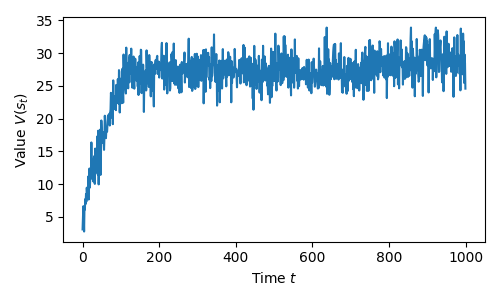
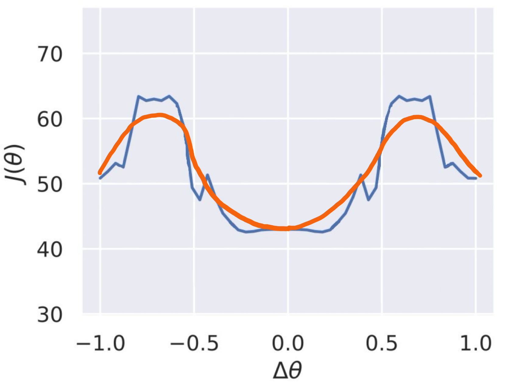
The second common pattern I found is that these cyclic tasks appear convex after stochastic smoothing (see my other blog post What makes RL tick). In one experiment, I took the converged optimal Anymal running policy and varied a single parameter in the actor neural network to generate a pseudo-landscape of the optimization problem. The orange line in the figure below sketches the appearance of the landscape after applying stochastic smoothing.

While the landscape is not convex, sufficient stochastic smoothing transforms it into a shape that most RL algorithms can handle effectively. This smoothing is one of the key factors enabling RL to tackle problems that classical control methods have struggled with for decades. In my experience, all cyclic tasks exhibit improved convexity after smoothing.

What can RL not do?

While RL often appears magical, in my opinion, it is terrible at non-cyclic tasks.

A simple example is the pick-and-place task. Sure, you might eventually get it to work, but no matter how much reward engineering you do, RL is fundamentally ill-suited for such tasks! Consider the well-engineered StackCube task from Maniskill3.

Their reward function is a whopping 36 lines of code! They have 3 modes of reward: (1) bring robot arm to cube to pick, (2) grasp cube on put on top of other cube, and (3) ungrasp cube. Here is a sketch of how I think that translates to a value function over time.

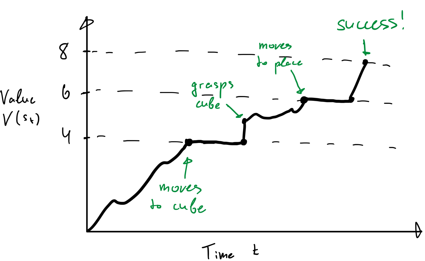
The optimization landscape in this case is highly non-trivial, with the RL algorithm oscillating between different task states. This makes the learning process significantly more challenging.

The focal example of this blog is the PushT task. It’s a contact-rich, highly non-convex task where a robot must push a T-shaped object into a goal pose. The success criteria is 95% overlap, and the straightforward reward is:

reward = clip(coverage / success_threshold, 0.0, 1.0)

Despite its apparent simplicity, this is an incredible hard task for RL. The core issue is that the task requires the agent to make and break contact at various positions, which traps the RL algorithm in the task’s inherent local minima. I experimented with TD-MPC2 [8]—an actor-critic method that leverages online planning—because it seemed the most promising. However, even after extensive tuning, it achieved a 0% success rate.

Why can’t RL solve it? To find out, let us investigate the optimization landscape for the actor \(J(a_t) = Q(s_t, a_t)\) where the actor is trying to find the action that maximizes the value function. By replaying an expert demonstration with the converged critic and sampling actions $a_t$ over the full range at each timestep, we can visualize the optimization landscape for RL.

Darker colors indicate high value (low loss), and light colors indicate low value (high loss). The cross is the action taken in the dataset. Pause and replay the video. Observe the times at which the agent has to break contact and go away from the object. These actions form local minima from which RL struggles to escape! Importantly, this isn’t a shortcoming of TD-MPC2 alone; even state-of-the-art algorithms like PPO and DreamerV3 face similar challenges on this seemingly simple task [3]. It appears that the RL problem formulation itself is mismatched with the nature of the task.

There’s another compounding issue. In the landscape above, I used a fixed critic, meaning the actor had a static objective. In practice, however, algorithms like TD-MPC2 update the actor and critic alternately, which results in a moving optimization target. From an optimization perspective, this is disastrous. The following video illustrates the evolving optimization landscape throughout the RL learning process:

Another fundamental problem is that RL optimization is painfully inefficient because it relies on zeroth-order gradients [10]. Since the environment is usually assumed to be unknown, we can’t compute gradients directly, limiting us to TD learning approaches that require vast amounts of data. Interestingly, even when the environment dynamics are learned, this does not necessarily speed up value function learning [11].

In summary, the fundamental issues with RL are:

1. RL is bad at non-cyclic tasks due to the natural local minima of the tasks.
2. The policy objective is a moving target, making learning unstable.
3. Reliance on zeroth-order gradients makes RL data-inefficient.

The beautiful simplicity of BC

If you’ve been around robotics, you’ve likely encountered the new cool kid on the block—Behavior Cloning (BC). While BC isn’t entirely new (see this 1989 paper), recent influential work like Diffusion Policy [4], OpenVLA [5], and $\pi_0$ [6] has achieved impressive manipulation tasks—such as folding T-shirts or picking up grapes from a plastic box with a spoon—directly from image observations. Meanwhile, RL still struggles with tasks like stacking cubes even when given privileged state information.

Why does BC succeed where RL has trouble? I believe it’s largely due to two reasons: (1) its inherent simplicity, and (2) the fact that supervised learning is generally easier to optimize than RL’s objective. To illustrate this, let’s examine one of the simplest yet impressive BC algorithms—the Action Chunking Transformer (ACT) [7]. The process is straightforward:

1. Collect some expert demonstration data (usually via teleoperation).
2. Get observation $o_t$ from your offline dataset.
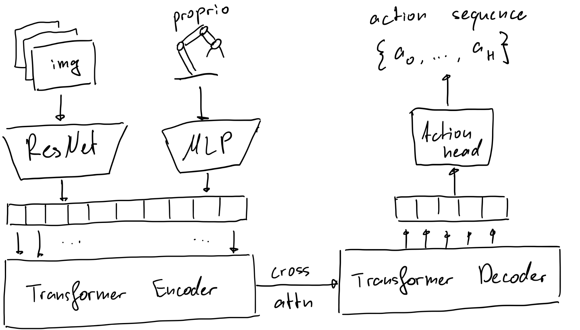
3. Tokenize images with a pretrained ResNet. Tokenize state data with an MLP.
4. Feed both into a transformer encoder-decoder to predict a trajectory \(\hat{A}_t = \pi_\theta (o_t)\) and train it to regress some ground truth (expert data) using supervised learning:

Below is a sketch of this elegant, streamlined architecture:

Using 200 expert demonstrations, I trained a simple ACT policy to solve the PushT task—achieving a 78% success rate (a dramatic improvement over RL’s 0% on this task).

Why does this work so much better, especially with such a simple algorithm? There are several reasons, but BC elegantly addresses the issues inherent in RL:

1. The objective is fully convex.
2. The objective is fixed.
3. The objective can be optimized efficiently with standard first-order gradient optimization.

To illustrate the convexity of the problem, here’s a visualization of the policy objective plotted over an expert demonstration:

Similar to before, darker shades indicate lower loss. How exciting! The smooth, continuous landscape—with no local minima—makes the optimization well-posed for non-cyclic tasks. Because the BC optimization problem is both simpler and more stable, it also allows us to scale up to higher-dimensional problems. This simplicity has been a key enabler for developing end-to-end policies directly from images.

That being said, BC isn’t perfect and it has it’s issues:

1. You must manually collect teleoperated demonstration data, which can be expensive. However, this cost is often much lower than dealing with the damage and downtime from RL experiments that break your robot.
2. By definition, BC can’t exceed the performance of the provided demonstrations. Yet, achieving a suboptimal solution is far preferable to a complete failure.

That being said, BC is simple and that is its greatest strength. I’ll leave you with a quote from a friend:

You can probably do everything that BC does with classical robotics methods. However, that would need a huge team of people collaborating for years to get any reasonable form of generalizability. Meanwhile, BC can achieve the same results with 3 people and a couple of weeks. The best part? Solving new tasks just involves adding more data!

Out of distribution

Whether it is a good idea or not, what works currently in robot learning is offline training. That is only natural for BC, and RL can still be applied in the form of offline RL. However, assessing Out of Distribution (OOD) performance in robotics is uniquely challenging. Even when operating within the known distribution, an action can push a robot into unfamiliar states. Going OOD in robotics isn’t just a theoretical concern—it can result in broken hardware or even put human safety at risk.

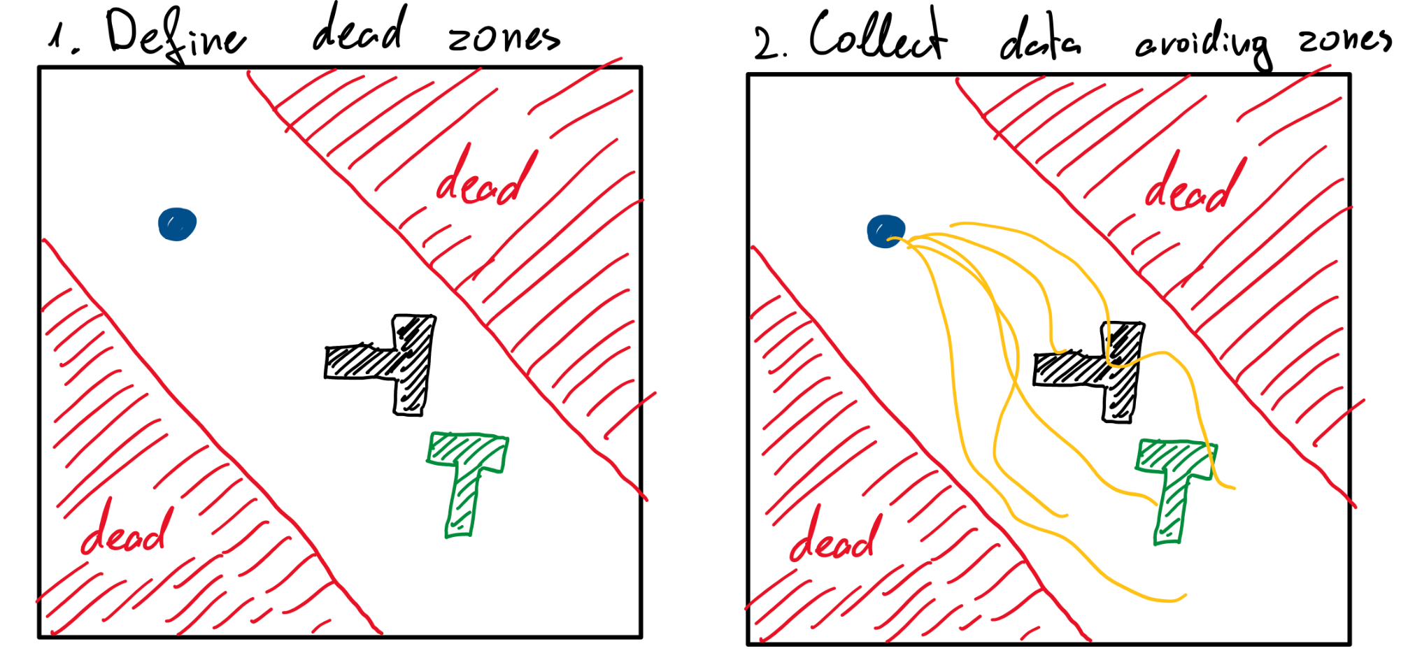
Let’s consider an imaginary experiment. Imagine a constrained version of the PushT task where if the robot approaches a certain corner, it “dies”, and replacing the robot is prohibitively expensive. Because of this, we cannot allow RL to train online; instead, we must rely on offline data collected by cautious human operators who naturally avoid dangerous regions. Then we use this data to offline train BC and RL. I collected 200 episodes and assumed that we always start in distribution (not realistic).

The case for BC is simple: as long as it remains in distribution, it will predict correctly and continue to stay in distribution. Naturally this gets harder as you get to more complex problems, but for our simple problem it holds surprisingly well! I trained ACT on this new dataset and got 84% task success rate and 2% death rate! Surprisingly, better than before! I suspect that is because I have limited my problem space and always start in-distribution. Thus, for our simple problem, BC works marvelously well!

RL, on the other hand, faces a tougher challenge. By its nature, RL must explore to find optimal solutions. In our hypothetical scenario, exploration can lead directly to death. In actor-critic architectures, this issue is particularly pronounced: the critic may erroneously assign high rewards to OOD states, while the actor—unfamiliar with these states—produces poor predictions. This creates a vicious cycle where the RL agent confidently “jumps off a cliff.” Here is a visualization of the problem landscape of TD-MPC2 offline trained on this task.

Similar to before, darker colors indicate higher value (lower loss) and lighter colors indicate low value (high loss). The red line indicate the death zone. The RL agent wants to go towards the dark regions and thus confidently jump off a cliff to its death. In my experiment, the RL approach achieved a 0% success rate and a 68% death rate over 50 evaluation episodes—a disastrous outcome that, if applied to a humanoid robot, could translate to six-figure losses.

Conclusion

Everybody wants to love RL. I want to love RL! However, I can’t ignore the simple elegance and performance of modern BC in robotics. In summary, these, in my opinion, are the pros and cons of BC vs. RL:

• ✅ Much simpler.
• ✅ The policy objective is convex and fixed.
• ✅ Can be optimized efficiently.
• ✅ Tends to stay in data distribution.
• ❌ Theoretically can’t surpass training data performance thus never optimal.
• ❌ Requires teleoperating your target robot.

Here is a direct comparison between the optimization landscapes of RL and BC. Ask yourself, which one do you want to solve?

There’s a huge race right now with multiple industry labs and startups pushing multi-task BC methods to their limits. The next few years will be exciting! Who knows, maybe RL will make a comeback just like it did with ChatGPT. It’s an exciting time to be in robotics!

Thank you for making it this far. I hope that you learned something!

If you have any comments or suggestions, shoot me an email!

Here are also some additional resources on this topic:

1. Sergey Levine’s lecture on supervised learning - sligthly updated but a great tutorial from the basics.
2. Abhishek Gupta’s lecture on RL - connects BC and RL nicely and comments on the issues of offline learning in robotics.

References

• [1] Rudin et al. Learning to Walk in Minutes Using Massively Parallel Deep Reinforcement Learning
• [2] Christopher et al. Limit Cycles of Differential Equations
• [3] Zhou et al. DINO-WM: World Models on Pre-trained Visual Features enable Zero-shot Planning
• [4] Chi et al. Diffusion Policy: Visuomotor Policy Learning via Action Diffusion
• [5] Kim et al. OpenVLA: An Open-Source Vision-Language-Action Model
• [6] Black et a. π0: A Vision-Language-Action Flow Model for General Robot Control
• [7] Zhao et al. Learning Fine-Grained Bimanual Manipulation with Low-Cost Hardware
• [8] Hansen et al. TD-MPC2: Scalable, Robust World Models for Continuous Control
• [9] Georgiev et al., Adaptive Horizon Actor-Critic for Policy Learning in Contact-Rich Differentiable Simulation
• [10] Mohamed et al., Monte Carlo Gradient Estimation in Machine Learning
• [11] Amos et al., On the model-based stochastic value gradient for continuous reinforcement learning